Lab 5

Linear PID Control and Linear Interpolation

Prelab

When I start my robot, I will send values to the Artemis, such as Kp and Ki, over Bluetooth by writing these values in the command on my Jupyter notebook. An example of the command I would send is: ble.send_command(CMD.COMMAND_NAME, "1|2|3"). This allows me to fine tune my closed loop controller without having to upload new code whenever I make any changes.

In my Arduino code, I need to add this to the beginning of the case to receive the inputs:

I will implement a time out in my code so the robot automatically stops after a defined amount of time. I will send this time out value over Bluetooth as well. This time out will always run regardless of Bluetooth connection.

I will initialize arrays when I run the controller and send these arrays to my computer over Bluetooth when the program is finished. The data that I’m collecting in these arrays are timestamps, sensor distance data, and outputs from the branches of the PID controller. The setup values will also be stored in variables and will be outputted after completion.

Task 1: Position Control

Since I am operating the ToF sensors in short range mode, the maximum range I can get is 1.3 meters (4.27 ft). If I start my robot 1.3 meters away from the wall and want to have the robot stop when it is 0.304 meters away, the maximum error I can expect is 0.996 meters. The values from the sensors is outputted in mm. Since the maximum PWM value I can apply to the motors is 255 for 100% speed, the maximum Kp value for this setup will be 255 / 996 mm = 0.256.

The final values I chosen for my PID controller are: Kp = 0.08, Ki = 0.60, and Kd = 0.05.

The reason why these values are very high is because my car has a lot of static friction for it to start rolling. I initially started with PI, but because of my large deadband value I had to implement for my robot, I was not able to make the robot stop 1 foot from the wall within 10 seconds. If my Ki was too low, my robot would stop early and far from the wall. If my Ki was too high, the robot would overshoot and hit the wall.

Because the error accumulates and continues to increase if the error stays positive, I had to implement a Kd term to counteract the integrator term. This allows the robot to slow down as it approaches the target distance, but also allows the integrator term to make final adjustments after the robot initially stops.

I implemented code to eliminate the initial derivative kick. When the derivative term compares the current error to the last error, the difference is very high for the first reading because the last error is initialized to 0. To solve this issue, I set the last error to be the same as the current error for the first calculation. The derivative term would be equal to 0 for the first calculation, and then calculates normally afterwards.

I included a low-pass filter to smooth out the changes in error. This is what the derivative term would have contributed to the PID controller if there is no low-pass filter (alpha = 1).

To smooth out the data, I used an alpha of 0.1.

Below is the full implementation of the PID controller:

Sensor sampling rate discussion

The sensor sampling rate must be fast enough relative to the PID loop rate so that each iteration of the controller receives a new measurement. If the sensor sampling rate is too slow, the controller may read the same value from the sensor across multiple iterations. Since the derivative term depends on the change in error between iterations, repeated measurements will cause the computed derivative to be zero during those iterations. When the sensor finally updates, the derivative term may produce a sudden spike because the accumulated change in error occurs in a single step. This reduces the effectiveness of the derivative term of the PID controller.

Results

I tested this PID controller at 3 different distances: 4 ft, 3 ft, and 2 ft.

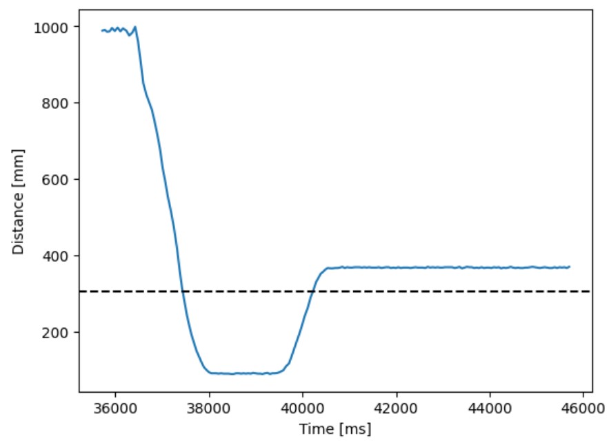
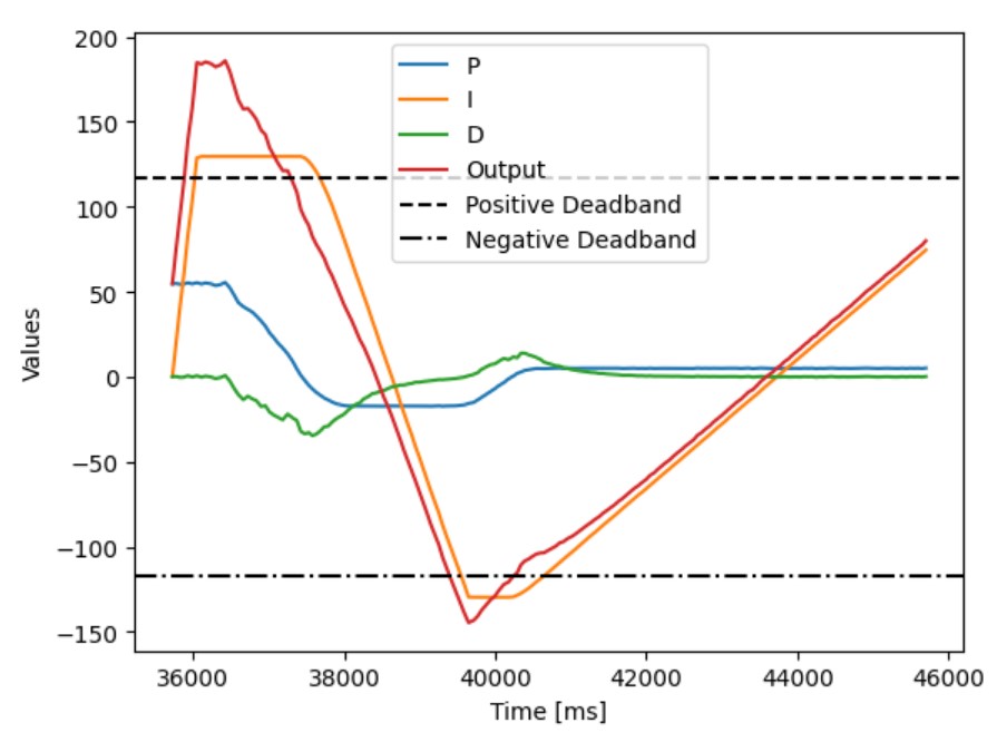
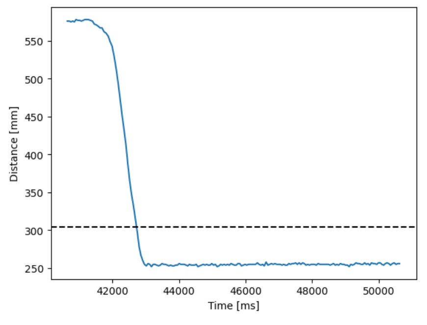
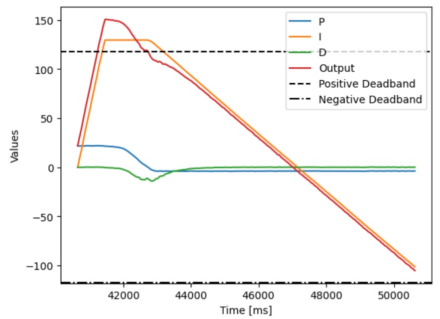
4 ft:

3 ft:

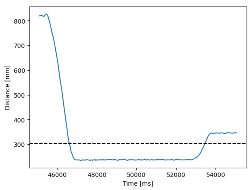
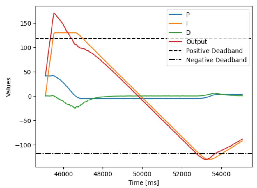
2 ft:

Maximum linear speed

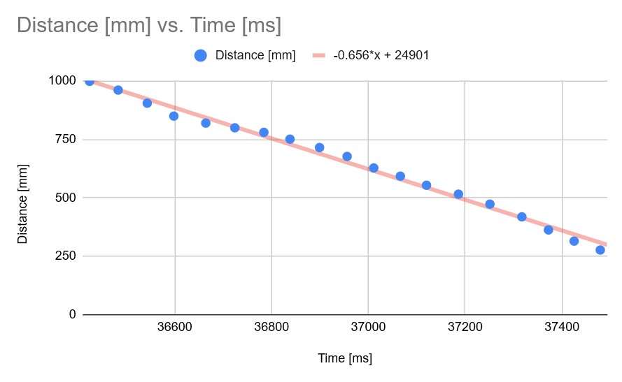
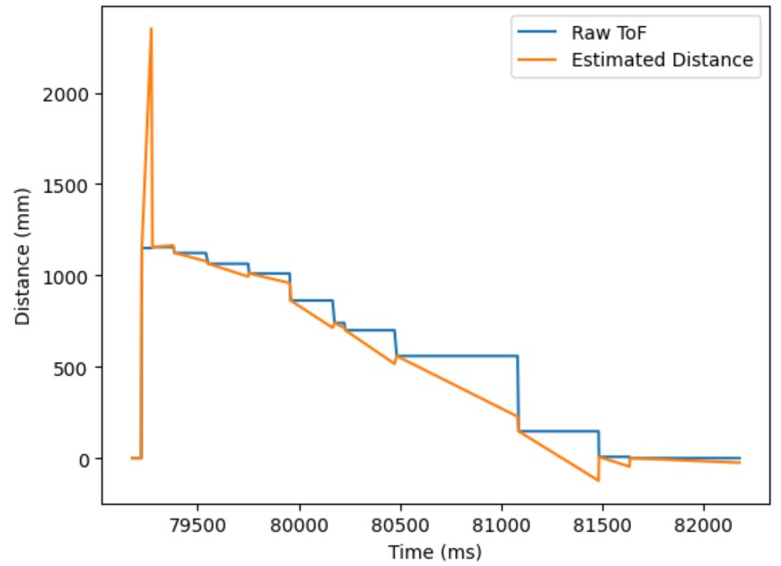
I did a linear interpolation on a portion of the distance-time data for 4 ft. The slope of the equation is -0.656 mm/ms, which equates to a maximum linear speed of 0.656 m/s.

Robust to external perturbations

To show that the PID controller is robust to external perturbations, I picked up the robot and placed it further from the wall, and then I picked it up again and placed it closer to the wall. Both times after I moved the robot, it moved toward the desired setpoint.

Task 2: Extrapolation

Looking at the time stamps between each data sample, the average time between each loop of the PID controller is (45700 - 35725) / 186 = 53.6 ms. This corresponds to a frequency of 18.6 Hz.

The following code snippet shows how I calculated the PID control every loop without checking for new data from the ToF sensor:

When running the new code for 3 seconds, the PID loop ran 704 times (234.7 Hz) while the distance only updated 13 times (4.3 Hz). The PID loop runs much faster than the distance sensor can update.

I used the following Python code to generate the extrapolated distances:

Tasks for 5000-level students

I implemented wind-up protection for the integrator. This is necessary because the total error accumulates and continues to increase when the error remains positive. This can cause the integrator term to be excessively large and can dominate over the Kp and Kd terms. To prevent the integrator term from over-saturating the controller, I clamped the integrator term if it exceeded the value of 130. This limits the integrator term to a maximum of ~51% speed to the controller. This value was found through experimental testing.

All three tests show that the Ki term saturates at the value of 130 for the wind-up protection.

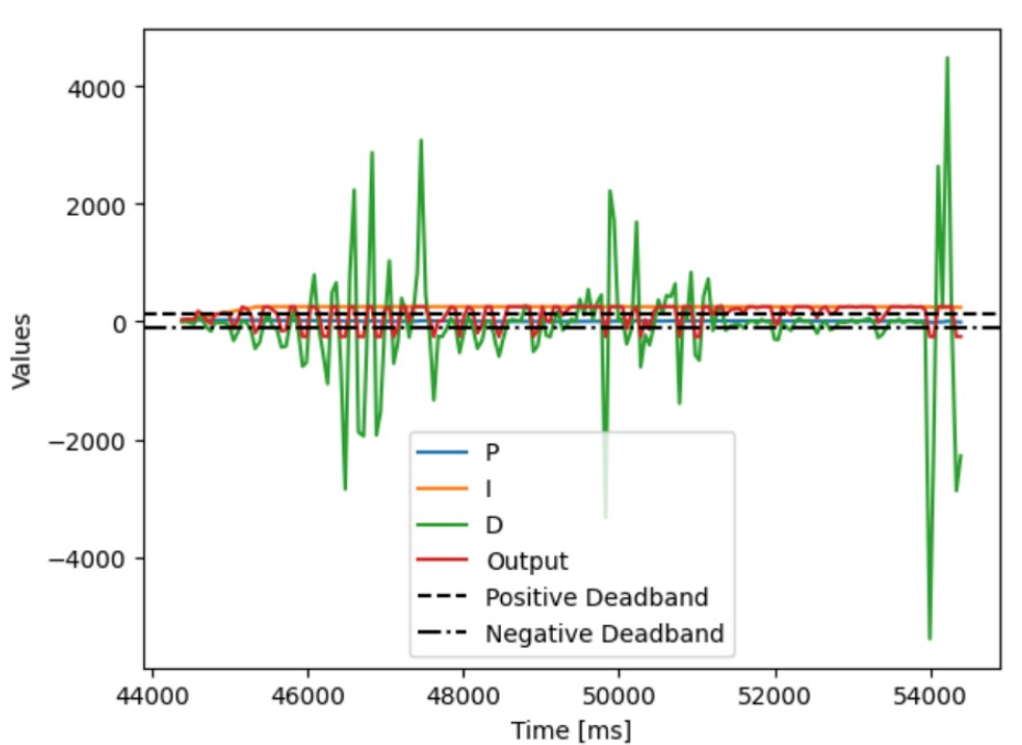
This is an example without wind-up protection at 4 ft:

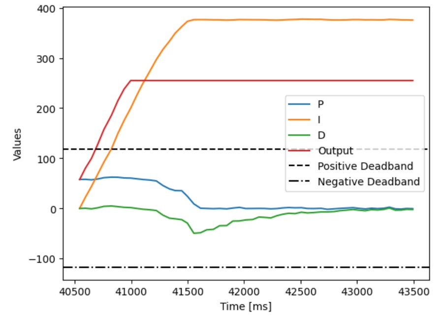
The output increases quickly and stays at the max PWM value of 255. For my robot, this causes it to not drive straight due to the large current draw by the motors. The robot requires wind-up protection to drive straight.

Collaborators

I collaborated with Sam Zhen while working on this lab.