Lab 12
Path Planning and Execution
Approach
The objective of this lab is to have the robot navigate through a sequence of waypoints in the environment as quickly and accurately as possible. My robot will use a combination of grid localization with Bayes filter and open-loop control. The robot used a ToF sensor to read and send ranging data and a gyroscope for orientation.
The approach followed a turn-go-turn paradigm. At each waypoint, the robot will:
- Perform a 360° observation and update its belief
- Compute the required heading and distance to next waypoint
- Perform an open-loop turn using gyroscope feedback
- Perform a straight drive using ToF distance readings
The entire path planning sequence is ran as a single code block on a Jupyter notebook. The robot automatically calculates the heading and distance to next target without any user inputs.
Waypoints
The waypoints were originally given in feet as grid cells. They were converted to meters to match the units for the Bayes filter and distance data.
| Waypoints | Grid [ft] | X [m] | Y [m] |
|---|---|---|---|
| 1 | (-4, -3) | -1.2192 | -0.9144 |
| 2 | (-2, -1) | -0.6096 | -0.3048 |
| 3 | (1, -1) | 0.3048 | -0.3048 |
| 4 | (2, -3) | 0.6096 | -0.9144 |
| 5 | (5, -3) | 1.524 | -0.9144 |
| 6 | (5, -2) | 1.524 | -0.6096 |
| 7 | (5, 3) | 1.524 | 0.9144 |
| 8 | (0, 3) | 0 | 0.9144 |
| 9 | (0, 0) | 0 | 0 |
The robot starts at waypoint 1 and attempted to visit each subsequent waypoint in order.
Code Overview
Below is a snippet of the code block that runs the entire path planning. The loc.get_observation_data() function is the same mapping command that was implemented in Lab 11. The robot performs a 360° turn to collect the 18 ToF readings, then the Jupyter notebook runs the Bayes filter update step. The most likely pose (cell with highest probability in loc.bel) is converted into (x, y, theta) coordinates using mapper.from_map(). The heading and distance to the next waypoint are calculated with angle_to_target() and distance_to_target().
Below are the helper functions used to calculate the heading and distance to the next waypoint. The heading angle is in degrees and the distance is in mm.
Below is the Arduino command for TURN_OPEN. The target_angle is calculated on the Jupyter notebook. The deadband is set to 1 degree. Turn factor is used to adjust the scaling of the gyroscope reading. The robot turns open-loop until it reaches the setpoint within the deadband.
Below is the Arduino command for DRIVE_TOF. The first distance reading is the reference reading. The robot drives forward while comparing the new distance reading to the reference. Once the difference between the current and reference readings is within the threshold of distance_to_travel, the robot stops.
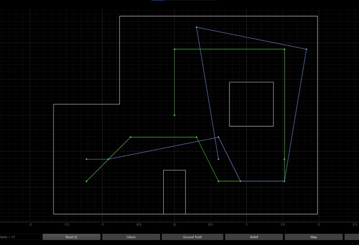
Video and Map of Path Planning
Bayes Filter Performance
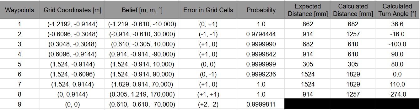
After each observation and update step, the Jupyter notebook logged the most probable grid cell, its probability, and the corresponding pose.
Discussion
The robot was able to traverse through the environment without hitting any of the walls while following relatively close to the intended path. For all but the last waypoint, the robot’s error was at most one grid cell in either the x or y directions. However for the last waypoint, the robot was 2 grid cells off in both the x and y directions. The belief was often offset by one grid cell in either x or y because the robot’s true pose falls near the boundary between two cells, but the discrete nature of the grid forces the belief to snap to the center of one cell. A smaller grid size can help with localization, but will increase computational time. A finer resolution will increase the number of cells the Bayes filter needs to compute probabilities for each one.
There were some general distance and turning errors based on the robot’s belief relative to where it was in the environment. For example, the robot’s belief for waypoint 2 was one cell to the left and one cell below the actual waypoint, even though the robot was close to the actual waypoint. The calculated distance for the robot to travel towards waypoint 3 was 1257 mm, much greater than the expected distance of 914 mm if the robot were directly on waypoint 2. This caused the robot to overshoot waypoint 3.
The Bayes filter consistently reported extremely high probabilities. This suggests the sensor noise parameter was likely set too low, causing the filter to become overconfident. Despite the high probabilities, the beliefs do not correspond to the robot’s actual physical location. This causes the robot to sometimes overshoot or miss short of the next waypoint. If the robot’s belief was very close to its actual location, it can travel to the next waypoint accurately (see waypoint 3 to 4 in the video).
The robot takes about 30 seconds to localize and update its belief before moving to the next waypoint. The entire sequence took 5.5 minutes.
To make the path planning more accurate in the future, I would try changing the sensor noise parameter and decreasing the grid cell size for more accurate poses.
Collaborators
N/A
Back to Labs